根据JPEG编码的流程,将一个JPEG编码的图像解码为YUV的原始像素图像。
实现了1x1宏块格式的解码,并输出为YUV444格式。
以Luc Saillard的jpeg_minidec作为范例。
由于没有时间仔细阅读JPEG标准,因此编写过程中借助范例调试对照了各个解码环节,并移植了范例中的部分代码到自己的项目中:
程序按照三个层次:
- BITIO提供文件/内存的比特流输入输出,比特流支持是为了适配Huffman解码的操作,方便逐比特读入数据。
- JPEG头解析和图像数据解码,包括文件头解析、Huffman解码 、IDCT等。
- 用户函数,包括加载JPEG文件,打印JPEG基本信息,解码,转码,保存几个主要函数。
另外还编写了一些用于调试的函数,如TRACE日志功能,用于跟踪打印程序调试输出。
JPEG格式解析
以下是JPEG编码的基本框图:
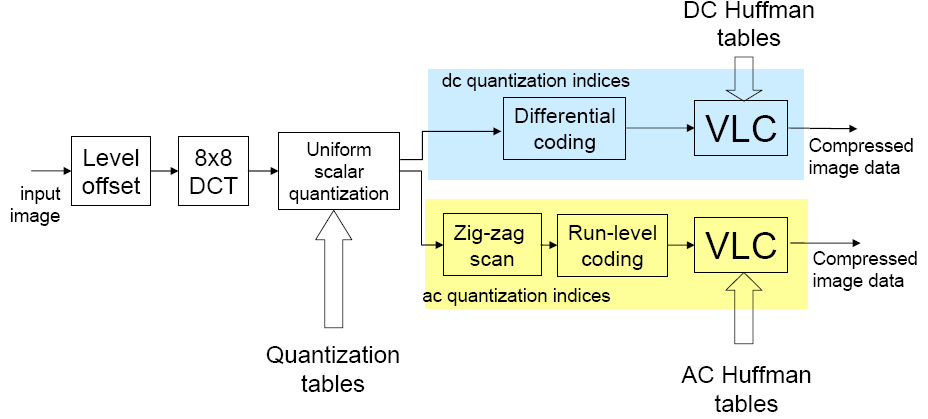 下面对编码过程做简要描述,重点是为了逆推解码过程。
- 零偏置
- 切分为若干的8x8宏块,并进行DCT变换得到8x8的DCT系数。
- 使用量化表对变换结果进行标量量化,DCT系数经量化后,取直流系数(直流系数为DCT系数的第一个),不同宏块之间的直流系数再经差分后再做Huffman编码。
- 对于交流系数,先经Zig-zag扫描(将有值的的数据集中到一起,提高游程编码和Huffman编码的效果),在进行游程编码和Huffman编码,得到最终的数据。
上面是编码过程的简要描述,没有涉及数据的具体存储方式,下面说一下解码的几个关键环节:
JPEG标记提取
JPEG标记有以下几种类型(摘自Wikipedia):
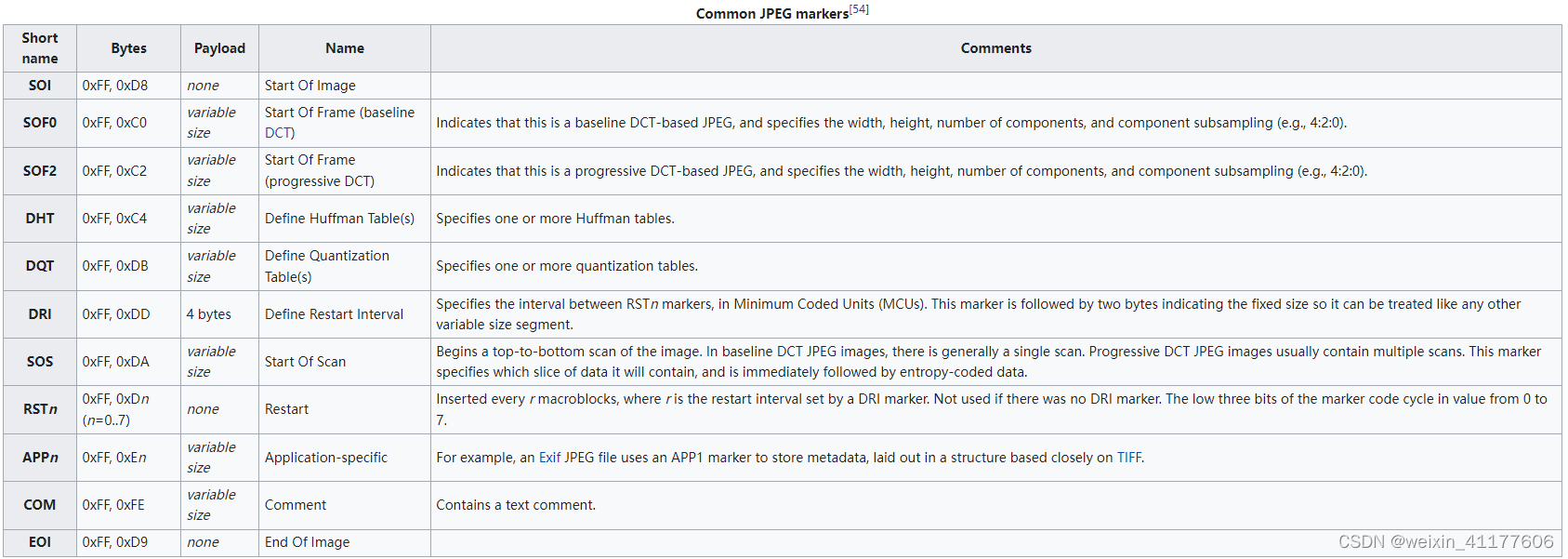 标记的起始格式是固定,第一个字节为0xff,第二个字节表明标记类型。
量化
图片自己会携带定义量化表(DQT)(两个,分别用于亮度分量和色度分量)作为参考量化表,将参考量化表再与JPEG规定的量化矩阵逐项相乘,得到用于转换的量化表。
DQT的结构为byte[64]
JPEG规定的量化表考虑了人眼视觉特性对不同频率分量的敏感特性:对低频敏感,对高频不敏感,因此对低频数据采用了细量化,对高频数据采用了粗量化。
static const double aanscalefactor[8] = {
   1.0, 1.387039845, 1.306562965, 1.175875602, 1.0, 0.785694958, 0.541196100, 0.275899379};
这是用到的量化表的参数值,从左到右分别对应8x8DCT变换后的直流、低频到高频系数,可以看到越到高频越倾向于将数值缩小(这样量化得到的系数越接近0),对于低频处的系数,倾向于放大数值,以实现比较精细的量化(在后续计算中降低舍入误差)。
下面是从定义量化表(DQT)构建最终可用的量化表的方式(取自jpeg_minidec)
void jpeg_build_quantization_table(float *qtable, byte * ref_table) {
    int i, j;
    static const double aanscalefactor[8] = {
        1.0, 1.387039845, 1.306562965, 1.175875602,
        1.0, 0.785694958, 0.541196100, 0.275899379};
    const unsigned char *zz = zigzag;

    for (i = 0; i < 8; i++)
    {
        for (j = 0; j < 8; j++)
        {
            *qtable++ = ref_table[*zz++] * aanscalefactor[i] * aanscalefactor[j];
        }
    }
}
Huffman编码
图片会携带定义Huffman表(DHT),共4个,分别用于亮度信号的直流、交流编码和色度信号的直流、交流编码。每个DHT会有一个自己编号,表明自己用于哪个信号的编码。
每个DHT有两个数组
- BitTable,指明了不同长度的码字的个数。BitTable所有值的总和即为用到的码字的个数(亦即下面ValueTable的长度),根据不同长度的码字个数,可以将码字逐个生成出来。
- ValueTable,每一个码字都对应一个权重(weight),这些权重值存储在ValueTable。权重值在直流、交流解码时有不同的意义。
由BitTable生成Huffman码字:
- 第一个码字必定为0
- 如果第一个码字位数为1,则码字为0
- 如果第二个码字位数为2,则码字为00,以此类推
- 从第二码字开始,如果它和它前面的码字位数相同,则当前码字为它前面的码字加1;如果它的位数比它前面的码字位数大,则当前码字的前面的码字加1后再在后面若干个零,直至满足位数长度为止。
下面给出了上述方法的具体实现(各种结构体的定义见源码):
void jpeg_build_huff_table(DHTInfo *dht_info) {
    HuffLookupTable * table = &dht_info->huff_table;
    int sum = 0;
    for(int i=0;i<16;i++){
        byte t = dht_info->bit_table[i];
        sum += t;
    };

    table->code = (word *) malloc(sizeof(word) * sum);
    table->len = (byte *) malloc(sizeof(byte) * sum);
    table->weight = (byte *) malloc(sizeof(byte) * sum);
    table->size = sum;

    // 生成Huffman表
    word code = 0;
    int idx = 1;
    int weight_idx = 0;
    for(int i=0;i<16;i++)
    {
        int n = dht_info->bit_table[i];

        if(n>0) idx++;
        for(int j=0;j<n;j++) {
            byte weight = dht_info->value_table[weight_idx];
            table->code[weight_idx] = code;
            table->len[weight_idx] = i+1;
            table->weight[weight_idx] = weight;
            code += 1;
            weight_idx += 1;
        }
        if(idx>1) code = (code)<<1;
    }
}
为了思路的简洁和方便实现,没有使用树/查找表等数据结构以提高查找速度。而是直接建立了码长-Huffman的对照表,当查找某个码长下的Huffman值,先跳到对应码长的码字部分,然后依次比对该码长下的码字,找到长度、值均相同的码字后,返回码字对应的权重值。这样虽然不够快,但是还可以接受。
以下是在Huffman表中查找某个码字的方法
byte jpeg_find_huff_code(DHTInfo *dht_info, int len, word code) {
    HuffLookupTable *table = &dht_info->huff_table;

    for(int i=0;i<table->size;i++) {
        int find_len = table->len[i];
        if(find_len==len) {
            if(table->code[i]==code) {
                return table->weight[i];
            }
            continue;
        } else if(find_len>len) break;
    }
    return 0xff;
}
下面是逐比特读出码字,然后在Huffman表中查找码字,如果码字不存在,就再读入一个比特继续查找,如果查找码长超过16bit,认为出错。
byte huffman_data_read(BITIO * input_stream, DHTInfo * dht){
    BITIO *bitio = input_stream;
    word b = read_bit(bitio)<<1;
    byte weight;
    int j = 0;
    for (j = 2; j <= 16; j++)
    {
        word k = read_bit(bitio);
        b =  b + k;

        weight = jpeg_find_huff_code(dht, j, b);

        b = b<<1;
        if (weight != 0xff) break;
    }
    ASSERT((weight!=0xff), "Huffman code not found!", TRACE_CONTENT("Test "BYTE_TO_BINARY_PATTERN, BYTE_TO_BINARY(b)));
    //TRACE_DEBUG("b="BYTE_TO_BINARY_PATTERN"_"BYTE_TO_BINARY_PATTERN"(%d) word=%d weight=%d", BIN(b>>9), BIN(b>>1), j, b, weight);
    return weight;
}
权重值低四位指明了需要再读几个比特以得到实际数值。权重值的高四位则指明了游程编码的游程长度,表明该数值后的连续几个DCT系数均为0。
直流系数没有游程编码,因此高四位始终为0。
读取的数个比特得到的实际上是有符号数,将其转换成定长的两字节有符号整形的方法是:(取自jpeg_minidec)
short bits;
bits = read_bits();
if ((word)bits < (1UL<<((bits_n)-1)))
    bits += (0xFFFFUL<<(bits_n))+1;
反量化&IDCT变换
以下是反量化同时做IDCT变换的代码实现(取自jpeg_minidec),因为是固定的8x8IDCT,所以作者采用了比较直接的计算方式。
/*
* Perform dequantization and inverse DCT on one block of coefficients.
*/
void
tinyjpeg_idct_float (short * DCT, float *Q_table, byte *output_buf, int stride)
{
FAST_FLOAT tmp0, tmp1, tmp2, tmp3, tmp4, tmp5, tmp6, tmp7;
FAST_FLOAT tmp10, tmp11, tmp12, tmp13;
FAST_FLOAT z5, z10, z11, z12, z13;
short *inptr;
FAST_FLOAT *quantptr;
FAST_FLOAT *wsptr;
byte *outptr;
int ctr;
FAST_FLOAT workspace[DCTSIZE2]; /* buffers data between passes */
/* Pass 1: process columns from input, store into work array. */
inptr = DCT;
quantptr = Q_table;
wsptr = workspace;
for (ctr = DCTSIZE; ctr > 0; ctr--) {
/* Due to quantization, we will usually find that many of the input
* coefficients are zero, especially the AC terms. We can exploit this
* by short-circuiting the IDCT calculation for any column in which all
* the AC terms are zero. In that case each output is equal to the
* DC coefficient (with scale factor as needed).
* With typical images and quantization tables, half or more of the
* column DCT calculations can be simplified this way.
*/
if (inptr[DCTSIZE*1] == 0 && inptr[DCTSIZE*2] == 0 &&
inptr[DCTSIZE*3] == 0 && inptr[DCTSIZE*4] == 0 &&
inptr[DCTSIZE*5] == 0 && inptr[DCTSIZE*6] == 0 &&
inptr[DCTSIZE*7] == 0) {
/* AC terms all zero */
FAST_FLOAT dcval = DEQUANTIZE(inptr[DCTSIZE*0], quantptr[DCTSIZE*0]);
wsptr[DCTSIZE*0] = dcval;
wsptr[DCTSIZE*1] = dcval;
wsptr[DCTSIZE*2] = dcval;
wsptr[DCTSIZE*3] = dcval;
wsptr[DCTSIZE*4] = dcval;
wsptr[DCTSIZE*5] = dcval;
wsptr[DCTSIZE*6] = dcval;
wsptr[DCTSIZE*7] = dcval;
inptr++; /* advance pointers to next column */
quantptr++;
wsptr++;
continue;
}
/* Even part */
tmp0 = DEQUANTIZE(inptr[DCTSIZE*0], quantptr[DCTSIZE*0]);
tmp1 = DEQUANTIZE(inptr[DCTSIZE*2], quantptr[DCTSIZE*2]);
tmp2 = DEQUANTIZE(inptr[DCTSIZE*4], quantptr[DCTSIZE*4]);
tmp3 = DEQUANTIZE(inptr[DCTSIZE*6], quantptr[DCTSIZE*6]);
tmp10 = tmp0 + tmp2; /* phase 3 */
tmp11 = tmp0 - tmp2;
tmp13 = tmp1 + tmp3; /* phases 5-3 */
tmp12 = (tmp1 - tmp3) * ((FAST_FLOAT) 1.414213562) - tmp13; /* 2*c4 */
tmp0 = tmp10 + tmp13; /* phase 2 */
tmp3 = tmp10 - tmp13;
tmp1 = tmp11 + tmp12;
tmp2 = tmp11 - tmp12;
/* Odd part */
tmp4 = DEQUANTIZE(inptr[DCTSIZE*1], quantptr[DCTSIZE*1]);
tmp5 = DEQUANTIZE(inptr[DCTSIZE*3], quantptr[DCTSIZE*3]);
tmp6 = DEQUANTIZE(inptr[DCTSIZE*5], quantptr[DCTSIZE*5]);
tmp7 = DEQUANTIZE(inptr[DCTSIZE*7], quantptr[DCTSIZE*7]);
z13 = tmp6 + tmp5; /* phase 6 */
z10 = tmp6 - tmp5;
z11 = tmp4 + tmp7;
z12 = tmp4 - tmp7;
tmp7 = z11 + z13; /* phase 5 */
tmp11 = (z11 - z13) * ((FAST_FLOAT) 1.414213562); /* 2*c4 */
z5 = (z10 + z12) * ((FAST_FLOAT) 1.847759065); /* 2*c2 */
tmp10 = ((FAST_FLOAT) 1.082392200) * z12 - z5; /* 2*(c2-c6) */
tmp12 = ((FAST_FLOAT) -2.613125930) * z10 + z5; /* -2*(c2+c6) */
tmp6 = tmp12 - tmp7; /* phase 2 */
tmp5 = tmp11 - tmp6;
tmp4 = tmp10 + tmp5;
wsptr[DCTSIZE*0] = tmp0 + tmp7;
wsptr[DCTSIZE*7] = tmp0 - tmp7;
wsptr[DCTSIZE*1] = tmp1 + tmp6;
wsptr[DCTSIZE*6] = tmp1 - tmp6;
wsptr[DCTSIZE*2] = tmp2 + tmp5;
wsptr[DCTSIZE*5] = tmp2 - tmp5;
wsptr[DCTSIZE*4] = tmp3 + tmp4;
wsptr[DCTSIZE*3] = tmp3 - tmp4;
inptr++; /* advance pointers to next column */
quantptr++;
wsptr++;
}
/* Pass 2: process rows from work array, store into output array. */
/* Note that we must descale the results by a factor of 8 == 2**3. */
wsptr = workspace;
outptr = output_buf;
for (ctr = 0; ctr < DCTSIZE; ctr++) {
/* Rows of zeroes can be exploited in the same way as we did with columns.
* However, the column calculation has created many nonzero AC terms, so
* the simplification applies less often (typically 5% to 10% of the time).
* And testing floats for zero is relatively expensive, so we don't bother.
*/
/* Even part */
tmp10 = wsptr[0] + wsptr[4];
tmp11 = wsptr[0] - wsptr[4];
tmp13 = wsptr[2] + wsptr[6];
tmp12 = (wsptr[2] - wsptr[6]) * ((FAST_FLOAT) 1.414213562) - tmp13;
tmp0 = tmp10 + tmp13;
tmp3 = tmp10 - tmp13;
tmp1 = tmp11 + tmp12;
tmp2 = tmp11 - tmp12;
/* Odd part */
z13 = wsptr[5] + wsptr[3];
z10 = wsptr[5] - wsptr[3];
z11 = wsptr[1] + wsptr[7];
z12 = wsptr[1] - wsptr[7];
tmp7 = z11 + z13;
tmp11 = (z11 - z13) * ((FAST_FLOAT) 1.414213562);
z5 = (z10 + z12) * ((FAST_FLOAT) 1.847759065); /* 2*c2 */
tmp10 = ((FAST_FLOAT) 1.082392200) * z12 - z5; /* 2*(c2-c6) */
tmp12 = ((FAST_FLOAT) -2.613125930) * z10 + z5; /* -2*(c2+c6) */
tmp6 = tmp12 - tmp7;
tmp5 = tmp11 - tmp6;
tmp4 = tmp10 + tmp5;
/* Final output stage: scale down by a factor of 8 and range-limit */
outptr[0] = descale_and_clamp((int)(tmp0 + tmp7), 3);
outptr[7] = descale_and_clamp((int)(tmp0 - tmp7), 3);
outptr[1] = descale_and_clamp((int)(tmp1 + tmp6), 3);
outptr[6] = descale_and_clamp((int)(tmp1 - tmp6), 3);
outptr[2] = descale_and_clamp((int)(tmp2 + tmp5), 3);
outptr[5] = descale_and_clamp((int)(tmp2 - tmp5), 3);
outptr[4] = descale_and_clamp((int)(tmp3 + tmp4), 3);
outptr[3] = descale_and_clamp((int)(tmp3 - tmp4), 3);
wsptr += DCTSIZE; /* advance pointer to next row */
outptr += stride;
}
}
MCU的具体存放
SOS(Start of scan)段,存放了三个分量(Y,Cb,Cr)所用到的量化表号,
[INFO] @no.82   SOS Start Of Scan
[INFO] @no.83           - Comps: 3
[INFO] @no.88           - CompId:1  AC:0 DC:0
[INFO] @no.88           - CompId:2  AC:1 DC:1
[INFO] @no.88           - CompId:3  AC:1 DC:1
在SOS段尾部,会有3个字节:0x00 0x3f 0x00,这三个字节虽然各有含义(谱选择开始、谱选择结束,谱选择结束),但实际上在基本JPEG里就是固定的。在调试过程中,可以用这3个字节在编辑器里定位压缩数据的起始位置。
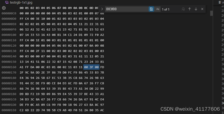
3个字节结束后,就是压缩图像数据,也就是一个一个MCU块。
从图像左上角到右下角的8x8MCU块在压缩图像数据中依次存放,每个MCU块内,Y、Cb、Cr三个分量分开依次存放:
[---------Y----------][---------Cb---------][-----------Cr-----------][---------Y----------][---------Cb---------][-----------Cr-----------]
下面给出了读取一个MCU块的一个分量的具体实现:
void jpeg_decode_mcu_huffman(DecodeHandler *handler, short * DCT)
{
BITIO * bitio = handler->input_stream;
byte weight = huffman_data_read(bitio, handler->dc_dht);
ASSERT(weight<=16, "Weight value error");
short DCT_r[64];
memset(DCT_r, 0, sizeof(DCT_r));
DCT_r[0] = read_bits_signed(bitio, weight);
DCT_r[0] += handler->prev_dc;
handler->prev_dc = DCT_r[0];
int j=1;
while(j<64) {
weight = huffman_data_read(bitio, handler->ac_dht);
byte size_val = weight & 0x0f;
byte count_0 = weight >> 4;
//TRACE_DEBUG("(%d) weight=%.2x size_val=%d count_0=%d", j+1, weight, size_val, count_0);
if(size_val == 0) {
if(count_0 == 0) {
//TRACE_DEBUG("EOB found");
break;
} else if(count_0 == 0x0f) {
j += 16; // skip 16 zeros
}
} else {
j += count_0;
ASSERT(j<64, "Bad huffman data (buffer overflow)");
short s = read_bits_signed(bitio, size_val);
DCT_r[j] = s;
//TRACE_DEBUG("DCT[%d]=%d", j, s);
j++;
}
}
for(int i=0;i<64;i++) {
DCT[i] = DCT_r[zigzag[i]];
}
}
解码效果
解码示例1
示例JPEG图片
![]()
执行
./build/Main ./test_images/testrgb-1x1.jpg ./test_output/output.yuv
进行解码。
打印日志输出(保留了INFO级别,输出中主要是解析得到的JPEG标志)
[INFO] @no.203  SOI: Start of Image
[INFO] @no.204  APP0 Application specific
[INFO] @no.207  DQT Define Quantization Table
[INFO] @no.207  DQT Define Quantization Table
[INFO] @no.208  SOF0 Start of Frame
[INFO] @no.209  DHT Define Huffman Tables
[INFO] @no.209  DHT Define Huffman Tables
[INFO] @no.209  DHT Define Huffman Tables
[INFO] @no.209  DHT Define Huffman Tables
[INFO] @no.210  SOS Start Of Scan
[INFO] @no.117  Print jpeg structure.
[INFO] @no.5    APP0 Application specific
[INFO] @no.6            - format: JFIF
[INFO] @no.7            - mVer: 1, sVer: 1
[INFO] @no.8            - unit: 0, x_den: 1, y_den: 1
[INFO] @no.9            - thumb: x: 0, y: 0
[INFO] @no.14   APP2 Application specific
[INFO] @no.15           - APP2 Length: 0
[INFO] @no.94   DQT Define Quantization Table
[INFO] @no.98           - DQT precious: 0 id: 0
[INFO] @no.100          - INDEX VALUE
[INFO] @no.103            0 2.0000
[INFO] @no.103            1 1.3870
[INFO] @no.103            2 1.3066
[INFO] @no.103            3 2.3518
[INFO] @no.103            4 2.0000
[INFO] @no.103            5 3.1428
[INFO] @no.103            6 2.7060
[INFO] @no.103            7 1.6554
[INFO] @no.103            8 1.3870
[INFO] @no.103            9 1.9239
[INFO] @no.103            10    1.8123
[INFO] @no.103            11    3.2620
[INFO] @no.103            12    4.1611
[INFO] @no.103            13    6.5387
[INFO] @no.103            14    4.5040
[INFO] @no.103            15    2.2961
[INFO] @no.103            16    1.3066
[INFO] @no.103            17    1.8123
[INFO] @no.103            18    3.4142
[INFO] @no.103            19    3.0727
[INFO] @no.103            20    5.2263
[INFO] @no.103            21    6.1594
[INFO] @no.103            22    4.9497
[INFO] @no.103            23    2.1629
[INFO] @no.103            24    1.1759
[INFO] @no.103            25    3.2620
[INFO] @no.103            26    3.0727
[INFO] @no.103            27    4.1481
[INFO] @no.103            28    5.8794
[INFO] @no.103            29    8.3149
[INFO] @no.103            30    5.0910
[INFO] @no.103            31    1.9465
[INFO] @no.103            32    2.0000
[INFO] @no.103            33    2.7741
[INFO] @no.103            34    5.2263
[INFO] @no.103            35    7.0553
[INFO] @no.103            36    7.0000
[INFO] @no.103            37    8.6426
[INFO] @no.103            38    5.4120
[INFO] @no.103            39    2.2072
[INFO] @no.103            40    1.5714
[INFO] @no.103            41    4.3592
[INFO] @no.103            42    6.1594
[INFO] @no.103            43    5.5433
[INFO] @no.103            44    6.2856
[INFO] @no.103            45    6.1732
[INFO] @no.103            46    4.6774
[INFO] @no.103            47    1.9510
[INFO] @no.103            48    2.7060
[INFO] @no.103            49    4.5040
[INFO] @no.103            50    5.6569
[INFO] @no.103            51    5.7274
[INFO] @no.103            52    5.4120
[INFO] @no.103            53    5.1026
[INFO] @no.103            54    3.5147
[INFO] @no.103            55    1.4932
[INFO] @no.103            56    1.9313
[INFO] @no.103            57    3.4442
[INFO] @no.103            58    3.6048
[INFO] @no.103            59    3.2442
[INFO] @no.103            60    3.0349
[INFO] @no.103            61    2.1677
[INFO] @no.103            62    1.4932
[INFO] @no.103            63    0.7612
[INFO] @no.94   DQT Define Quantization Table
[INFO] @no.98           - DQT precious: 0 id: 1
[INFO] @no.100          - INDEX VALUE
[INFO] @no.103            0 2.0000
[INFO] @no.103            1 2.7741
[INFO] @no.103            2 2.6131
[INFO] @no.103            3 5.8794
[INFO] @no.103            4 10.0000
[INFO] @no.103            5 7.8569
[INFO] @no.103            6 5.4120
[INFO] @no.103            7 2.7590
[INFO] @no.103            8 2.7741
[INFO] @no.103            9 3.8478
[INFO] @no.103            10    5.4368
[INFO] @no.103            11    11.4169
[INFO] @no.103            12    13.8704
[INFO] @no.103            13    10.8979
[INFO] @no.103            14    7.5066
[INFO] @no.103            15    3.8268
[INFO] @no.103            16    2.6131
[INFO] @no.103            17    5.4368
[INFO] @no.103            18    10.2426
[INFO] @no.103            19    15.3636
[INFO] @no.103            20    13.0656
[INFO] @no.103            21    10.2656
[INFO] @no.103            22    7.0711
[INFO] @no.103            23    3.6048
[INFO] @no.103            24    5.8794
[INFO] @no.103            25    11.4169
[INFO] @no.103            26    15.3636
[INFO] @no.103            27    13.8268
[INFO] @no.103            28    11.7588
[INFO] @no.103            29    9.2388
[INFO] @no.103            30    6.3638
[INFO] @no.103            31    3.2442
[INFO] @no.103            32    10.0000
[INFO] @no.103            33    13.8704
[INFO] @no.103            34    13.0656
[INFO] @no.103            35    11.7588
[INFO] @no.103            36    10.0000
[INFO] @no.103            37    7.8569
[INFO] @no.103            38    5.4120
[INFO] @no.103            39    2.7590
[INFO] @no.103            40    7.8569
[INFO] @no.103            41    10.8979
[INFO] @no.103            42    10.2656
[INFO] @no.103            43    9.2388
[INFO] @no.103            44    7.8569
[INFO] @no.103            45    6.1732
[INFO] @no.103            46    4.2522
[INFO] @no.103            47    2.1677
[INFO] @no.103            48    5.4120
[INFO] @no.103            49    7.5066
[INFO] @no.103            50    7.0711
[INFO] @no.103            51    6.3638
[INFO] @no.103            52    5.4120
[INFO] @no.103            53    4.2522
[INFO] @no.103            54    2.9289
[INFO] @no.103            55    1.4932
[INFO] @no.103            56    2.7590
[INFO] @no.103            57    3.8268
[INFO] @no.103            58    3.6048
[INFO] @no.103            59    3.2442
[INFO] @no.103            60    2.7590
[INFO] @no.103            61    2.1677
[INFO] @no.103            62    1.4932
[INFO] @no.103            63    0.7612
[INFO] @no.20   SOF0 Start of Frame
[INFO] @no.21           - Accur: 8
[INFO] @no.22           - Height: 1024, Width: 1024
[INFO] @no.23           - Comps: 3
[INFO] @no.27           - Comp Id: 1, sample: H:V=11, dqt: 0
[INFO] @no.27           - Comp Id: 2, sample: H:V=11, dqt: 1
[INFO] @no.27           - Comp Id: 3, sample: H:V=11, dqt: 1
[INFO] @no.34   DHT Define Huffman Tables
[INFO] @no.35           - DHT#0, DC
[INFO] @no.36           - BitTable: 00 03 01 01 01 01 01 01 01 00 00 00 00 00 00 00          (sum: 10)
[INFO] @no.48           - ValueTable: 04 05 06 03 02 01 00 09 07 08          (sum: 10)
[INFO] @no.64           + 00    0000000000000000(2) (4)
[INFO] @no.64           + 01    0000000000000001(2) (5)
[INFO] @no.64           + 02    0000000000000010(2) (6)
[INFO] @no.64           + 03    0000000000000110(3) (3)
[INFO] @no.64           + 04    0000000000001110(4) (2)
[INFO] @no.64           + 05    0000000000011110(5) (1)
[INFO] @no.64           + 06    0000000000111110(6) (0)
[INFO] @no.64           + 07    0000000001111110(7) (9)
[INFO] @no.64           + 08    0000000011111110(8) (7)
[INFO] @no.64           + 09    0000000111111110(9) (8)
[INFO] @no.34   DHT Define Huffman Tables
[INFO] @no.35           - DHT#1, DC
[INFO] @no.36           - BitTable: 00 03 01 01 01 01 01 01 01 01 00 00 00 00 00 00          (sum: 11)
[INFO] @no.48           - ValueTable: 04 05 06 03 02 01 00 07 0a 09 08       (sum: 11)
[INFO] @no.64           + 00    0000000000000000(2) (4)
[INFO] @no.64           + 01    0000000000000001(2) (5)
[INFO] @no.64           + 02    0000000000000010(2) (6)
[INFO] @no.64           + 03    0000000000000110(3) (3)
[INFO] @no.64           + 04    0000000000001110(4) (2)
[INFO] @no.64           + 05    0000000000011110(5) (1)
[INFO] @no.64           + 06    0000000000111110(6) (0)
[INFO] @no.64           + 07    0000000001111110(7) (7)
[INFO] @no.64           + 08    0000000011111110(8) (10)
[INFO] @no.64           + 09    0000000111111110(9) (9)
[INFO] @no.64           + 10    0000001111111110(10) (8)
[INFO] @no.34   DHT Define Huffman Tables
[INFO] @no.35           - DHT#0, AC
[INFO] @no.36           - BitTable: 00 01 02 05 03 03 03 02 05 03 04 02 02 02 01 05          (sum: 43)
[INFO] @no.48           - ValueTable: 00 01 03 02 04 05 11 21 22 31 61 06 12 a1 32 41 62 13 51 23 42 71 81 91 15 52 63 07 14 33 53 16 43 08 b1 34 c1 24 d1 09 72 f0 a2       (sum: 43)
[INFO] @no.64           + 00    0000000000000000(2) (0)
[INFO] @no.64           + 01    0000000000000010(3) (1)
[INFO] @no.64           + 02    0000000000000011(3) (3)
[INFO] @no.64           + 03    0000000000001000(4) (2)
[INFO] @no.64           + 04    0000000000001001(4) (4)
[INFO] @no.64           + 05    0000000000001010(4) (5)
[INFO] @no.64           + 06    0000000000001011(4) (17)
[INFO] @no.64           + 07    0000000000001100(4) (33)
[INFO] @no.64           + 08    0000000000011010(5) (34)
[INFO] @no.64           + 09    0000000000011011(5) (49)
[INFO] @no.64           + 10    0000000000011100(5) (97)
[INFO] @no.64           + 11    0000000000111010(6) (6)
[INFO] @no.64           + 12    0000000000111011(6) (18)
[INFO] @no.64           + 13    0000000000111100(6) (161)
[INFO] @no.64           + 14    0000000001111010(7) (50)
[INFO] @no.64           + 15    0000000001111011(7) (65)
[INFO] @no.64           + 16    0000000001111100(7) (98)
[INFO] @no.64           + 17    0000000011111010(8) (19)
[INFO] @no.64           + 18    0000000011111011(8) (81)
[INFO] @no.64           + 19    0000000111111000(9) (35)
[INFO] @no.64           + 20    0000000111111001(9) (66)
[INFO] @no.64           + 21    0000000111111010(9) (113)
[INFO] @no.64           + 22    0000000111111011(9) (129)
[INFO] @no.64           + 23    0000000111111100(9) (145)
[INFO] @no.64           + 24    0000001111111010(10) (21)
[INFO] @no.64           + 25    0000001111111011(10) (82)
[INFO] @no.64           + 26    0000001111111100(10) (99)
[INFO] @no.64           + 27    0000011111111010(11) (7)
[INFO] @no.64           + 28    0000011111111011(11) (20)
[INFO] @no.64           + 29    0000011111111100(11) (51)
[INFO] @no.64           + 30    0000011111111101(11) (83)
[INFO] @no.64           + 31    0000111111111100(12) (22)
[INFO] @no.64           + 32    0000111111111101(12) (67)
[INFO] @no.64           + 33    0001111111111100(13) (8)
[INFO] @no.64           + 34    0001111111111101(13) (177)
[INFO] @no.64           + 35    0011111111111100(14) (52)
[INFO] @no.64           + 36    0011111111111101(14) (193)
[INFO] @no.64           + 37    0111111111111100(15) (36)
[INFO] @no.64           + 38    1111111111111010(16) (209)
[INFO] @no.64           + 39    1111111111111011(16) (9)
[INFO] @no.64           + 40    1111111111111100(16) (114)
[INFO] @no.64           + 41    1111111111111101(16) (240)
[INFO] @no.64           + 42    1111111111111110(16) (162)
[INFO] @no.34   DHT Define Huffman Tables
[INFO] @no.35           - DHT#1, AC
[INFO] @no.36           - BitTable: 00 02 03 00 02 02 02 03 01 00 03 00 03 00 00 07          (sum: 28)
[INFO] @no.48           - ValueTable: 00 04 01 02 03 31 61 11 12 05 21 13 14 41 51 06 22 32 07 15 42 08 71 23 24 33 81 a1        (sum: 28)
[INFO] @no.64           + 00    0000000000000000(2) (0)
[INFO] @no.64           + 01    0000000000000001(2) (4)
[INFO] @no.64           + 02    0000000000000100(3) (1)
[INFO] @no.64           + 03    0000000000000101(3) (2)
[INFO] @no.64           + 04    0000000000000110(3) (3)
[INFO] @no.64           + 05    0000000000011100(5) (49)
[INFO] @no.64           + 06    0000000000011101(5) (97)
[INFO] @no.64           + 07    0000000000111100(6) (17)
[INFO] @no.64           + 08    0000000000111101(6) (18)
[INFO] @no.64           + 09    0000000001111100(7) (5)
[INFO] @no.64           + 10    0000000001111101(7) (33)
[INFO] @no.64           + 11    0000000011111100(8) (19)
[INFO] @no.64           + 12    0000000011111101(8) (20)
[INFO] @no.64           + 13    0000000011111110(8) (65)
[INFO] @no.64           + 14    0000000111111110(9) (81)
[INFO] @no.64           + 15    0000011111111100(11) (6)
[INFO] @no.64           + 16    0000011111111101(11) (34)
[INFO] @no.64           + 17    0000011111111110(11) (50)
[INFO] @no.64           + 18    0001111111111100(13) (7)
[INFO] @no.64           + 19    0001111111111101(13) (21)
[INFO] @no.64           + 20    0001111111111110(13) (66)
[INFO] @no.64           + 21    1111111111111000(16) (8)
[INFO] @no.64           + 22    1111111111111001(16) (113)
[INFO] @no.64           + 23    1111111111111010(16) (35)
[INFO] @no.64           + 24    1111111111111011(16) (36)
[INFO] @no.64           + 25    1111111111111100(16) (51)
[INFO] @no.64           + 26    1111111111111101(16) (129)
[INFO] @no.64           + 27    1111111111111110(16) (161)
[INFO] @no.82   SOS Start Of Scan
[INFO] @no.83           - Comps: 3
[INFO] @no.88           - CompId:1  AC:0 DC:0
[INFO] @no.88           - CompId:2  AC:1 DC:1
[INFO] @no.88           - CompId:3  AC:1 DC:1
[INFO] @no.403  Reach the end of the file
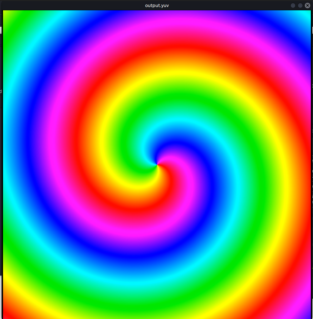
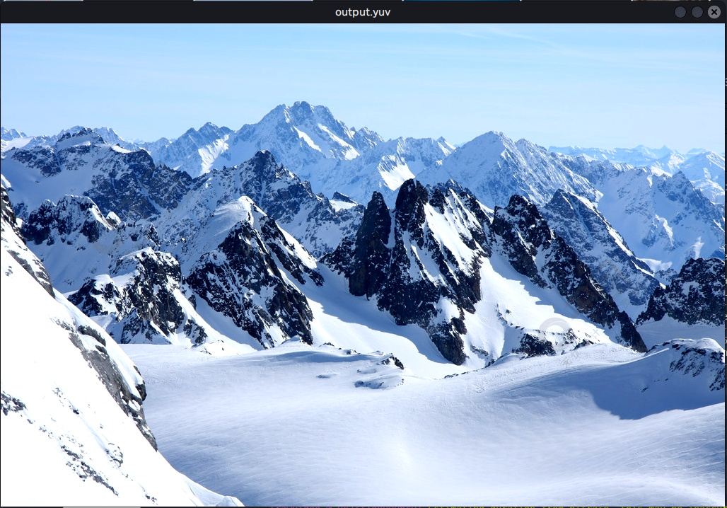
执行(需要安装FFmpeg, FFplay),显示解码得到的YUV文件
ffplay -video_size 1024x1024 -pixel_format yuv444p -i test_output/output.yuv
解码示例2
原图:
 解码结果:
解码结果:

可以看到下方有一条灰色未解码的区域,这是由于未考虑非8整数倍高度导致的。 对于高度非8整数倍的情况,处理比较简单,因为在MCU中,多出的边缘部分被置零,与实际存在的像素一起做DCT变换。 只需要将高度值向上增加至8整数倍进行解码,最后保存图片时,各个通道按实际高度保存即可。
// 调整至8整数倍
int expand_8(int value)
{
    if((value%8)==0) return value;
    else {
        return (value/8)*8 + 8;
    }
}
这样就避免了最后一部分未解码的情况,另一张非8整数倍高度的图片的解码效果(这张图片比较容易看清边缘的情况)
其他
最终得到的YUV444格式可以再作为源格式转换为YUV422/YUV420/RGB24等格式,在之前的实验中曾实现了这些格式之间的互转。
实验代码放在了
